Excel Vlookup Function - 3 Tutorial Videos With Examples

After watching these videos and reading the tutorial, you will get to fully understand how to use this function and the cases in which it is useful. It includes easy examples demonstrating the difference between finding an exact match and a close match. Also, you will see how you can use it to match lists and spot their differences.

Video: How to use the VLOOKUP function (exact match) Video: How to use the VLOOKUP function (closest match) Using Vlookup to Match Lists (And: Getting rid of the #N/A error)

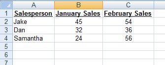
Let's assume we are given the following sales table:

If you wish to retrieve Dan's January sales (hence cell B3), the function will be:

Let's go over the different parts of the function in plain English (note the highlighted parts in the following sentence, taken out directly from the formula):
The function will look for the word "Dan" at the first (left) column of the range a2:c4. It will retrieve the value adjacent to it on the 2nd column (thus the "January" column).

The word "false" tells the function to find Exactly the word "Dan", and not something close or similar to it.

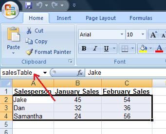
A way to make the function more readable is to name the table, and use this name in the vlookup function:
Select the table (no need to include the headers row), and write a name inside the name box (its located at the top left of the screen). In our vlookup example, we used the name "salesTable" (Try to avoid using spaces).

Thus, the function can now look like this:

And what if you don't want to retrieve always Dan's January sales, but to retrieve the name that will be written in cell A6?

And if you wish the function to retrieve February's sales (instead of January)?

When you have a table with data, and you wish to retrieve specific information from it.

Actually whenever you are looking up a name in a phone book, you are performing a “real” vlookup action: you look up the name of your recipient on the first (most left) column, and when finding it, you retrieve the number appearing next to that name.

An implementation of the vlookup in Excel could be:
You have an Excel table with student names and their grades.
You wish that you could somewhere in the sheet type a student name, and immediately retrieve his grade (based on the data in the table).
To achieve this, you can use "Vlookup": the function will look for the student’s name in the first column in the table, and will retrieve the information that is next to his name in the second column (which is his grade).

Check the video links above to learn how exactly this function is written and implemented inside the worksheet.

Another vlookup example:
You have a big table consisting thousands of bank accounts.
You wish to retrieve in another worksheet information regarding some specific accounts.
To achieve this, you can type these specific account numbers, and put a Vlookup function next each one of them. The function will look for the account numbers in the big table, and retrieve relevant information from it.

The difference between “Exact match” and “Closest match”:

When you use the Vlookup Excel function to retrieve information based on a student name or a bank account number, you cannot allow it to find something close or similar to “Jake”, or close to the account number “3647463”, but rather it has to find them exactly.

But sometimes you have a table that defines ranges, for example:
$5,000 – “Small deposit”
$20,000 – “Medium deposit”
$100,000 – “Big deposit”
$500,000 – “Huge deposit”

If you want the function to find the description for a deposit of $23,000 (which should retrieve “Medium deposit”), you will ask it to find a close match, and it will find $20,000.

This is very useful when dealing with dates. Look at the following table:
4/1/2008 – Payment on time.
6/1/2008 – Late with payment (small fine).
8/1/2008 – Very late with payment (big fine).

If you would like to find what happens with a payment made on 7/14/2008, the function will relate it to the date 6/1/2008 and retrieve us “Late with payment (small fine)”.

Please note – the function will always retrieve the smaller closest match (in case it doesn’t find an exact match).